Ⅰ. Introduction
In housing market, it is well known that there is a close relationship between housing prices and trading volume. For example, if we assume that there is positive correlation between housing prices and trading volume as well as the movement of trading volume leads that of housing prices, we can expect that trading volume increase will be followed by housing prices increase and trading volume decrease will be followed by housing prices decrease. If this happens, we could presume the future direction of housing price through checking the direction of trading volume in housing market.
For this reason, many studies have been conducted to confirm a close correlation or lead-lag relationship between housing prices and trading volume in long-term movements. Stein (1995) showed the research result that trading volume decreased when housing price decreased due to effects of down payment home owner paid. Genesove and Mayer (2001) also showed the phenomenon that trading volume decreased when housing price decreased, and asserted that although this phenomenon could not be explained by perfect asset market model but it could be explained by seller’s propensity of loss aversion or equity constraints. Clayton et al. (2010) showed that there was two-way Granger causation between housing prices and trading volume. Leung and Peng (2005) showed that there was one-way Granger causation from trading volume to housing prices in commercial building.
In the studies that analyzed Korean housing market. Lim (2011) showed that the causality appeared bidirectional and there was a positive correlation between housing prices and trading volume. Lim (2014) confirmed that a lead-lag relationship or co-movement between housing prices and trading volume had shown different results by region. Like these, the previous studies conducted to confirm the relationship between housing prices and trading volume mainly focused on a close correlation and lead-lag relationship in time domain.
Meanwhile, we can say that the movements of housing prices and trading volume have long-term cycles. So, we also can presume that there would be a close relationship between cyclic components embedded in these two variables. But, until now, it is difficult to find studies which analyzed cyclical characteristics and the relationship under common cycles embedded in these two variables.
In this analysis, unlike the previous studies conducted to confirm the correlation and lead-lag relationship between housing prices and trading volume using the methodologies in time domain analysis, we are trying to interpret from different points of view through analyzing cyclical characteristics embedded in these two variables by using spectral analysis in frequency domain. Through spectral analysis, we can show the lead-lag relationship between housing prices and trading volume under common cycles visually.1) After identifying common cycles embedded in these two variables, if we could confirm a close relationship under common cycles, it is expected that we could confirm the current position of two variables under long-term cycles and forecast future direction of the cycles.
When we forecast cycles in housing prices and trading volume, for the purpose of comparison, we added the results of VAR(p) model analysis in time domain in addition to the results of the spectral analysis in frequency domain. Ultimately, we could improve the rationality about the forecasting results of future cycles by confirming the results from time domain and frequency domain analysis concurrently. The paper is organized as follows. In Section 2, we briefly describe the methodology and data we use in our analysis. In Section 3, we describe the results of our analysis focusing on common cycles embedded in two variables. Finally, the paper is concluded in Section 4.
Ⅱ. Methodology and Data
To detect cycles in time series data, we can use the methodologies in frequency domain such as harmonic analysis, periodogram analysis, and spectral analysis. After detecting common cycles embedded in time series xt and yt, to confirm long-term relationship between these two time series under common cycles, we can conduct cross spectral analysis. Through the cross spectral analysis, we will obtain a squared coherence spectrum to estimate the percentage of shared variance between the two time series at a particular frequency band and we will also obtain a phase spectrum to estimate a phase relationship (or time lag) between the two time series within each frequency band (Wei, 1990; Warner, 1998). The squared coherence (Kxy(w)2) can be calculated as <Eq. 1> below.
Where, fxy(w): cross spectrum between xt and yt; fx(w): spectrum of xt; fy(w): spectrum of yt; w: angular frequency (2π/τ); τ: period or cycle length.
The phase (ϕxy(w)) can be calculated as <Eq. 2> below.
Where, −qxy(w): imaginary parts of fxy(w); cxy(w): real parts of fxy(w).
If we identify the cycles embedded in the time series using periodogram analysis, we could conduct harmonic analysis to show the identified cycle components visually. Harmonic analysis model for time series which includes sine (sin) and cosine (cos) functions can be expressed as <Eq. 3>.
Where, μ: mean value; t: observations (t=0, 1, …,N); εt: WN(0, σ2)
The formal model for the periodogram is an extension of the harmonic analysis model. As we can see in <Eq. 4>, the periodogram model represents the time series as a sum of N/2 periodic components.
Where, cos(wit): the cosine function of frequency wi; sin(wit): the sine function of frequency wi.
Periodogram analysis is a useful technique to search for hidden periodicities through assessing whether there is a strong cyclic component in a time series. Meanwhile, spectral analysis techniques were developed to reduce the possible problem of sampling error in periodogram analysis. An estimated power spectrum in the spectral analysis is a smoothed version of the periodogram. We use these smoothed spectrums for and when we calculate the squared coherence (Kxy(w)2) and the phase (ϕxy(w)) in the cross spectral analysis.
VAR(p) model allows for cross-variable dynamics. In an N-variable vector autoregression of order p (VAR(p)), we estimate N different equations. In VAR(p) model, each variable is related not only to its own past, but also to the past of all the other variables in the system. For example, we have two equations as in <Eq. 5> and <Eq. 6> in a two-variable VAR(p) model (Diebold, 2001).
This analysis was conducted to confirm the relationship between long-term cycles embedded in both growth rate of housing prices and trading volume. We can use monthly time series data of apartment price index and apartment trading volume from the database of Korea Real Estate Board2). To identify long-term cycles embedded in the time series, we used the year-on-year increase rates of apartment price index as the proxy variable of housing price change rates. And as the proxy variable of trading volume, we used the twelvemonth accumulated monthly apartment trading volume.
In this analysis, due to different characteristics of housing prices and trading volume by region, the region in our analysis is divided into four regions as follows. ① Total (Whole country), ② Seoul Metropolitan (Seoul, Incheon, Gyunggi), ③ 5 Big Cities (Busan, Daegu, Gwangju, Daejeon, Ulsan), ④ Non Metropolitan (Gangwon, Chungbuk, Chungnam, Jeonbuk, Jeonnam, Gyungbuk, Gyungnam, Jeju).
To find long-term relationship between housing price change rates and trading volume after identifying common cycles embedded in these two variables, we stabilized the pattern of time series of these two variables by eleminating the trends in these two variables using Hodrick-Prescott filtering method. As we can see from the Figures below, all modified variables show the pattern of fluctuating up and down centering around the mean value of zero. And then, we finally standardize these two variables to avoid the problem could be resulted from different units3).
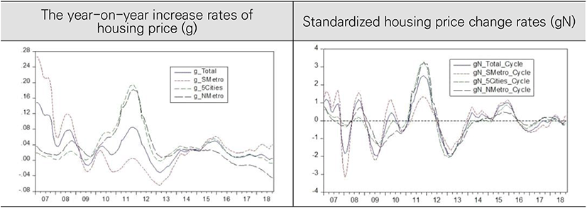
<Figure 1> show the year-on-year increase rates of housing price (g) and standardized housing price change rates (gN) by regions from 01.2007 to 10.2018.
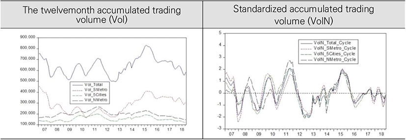
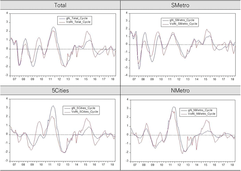
We could confirm that the cycles in the standardized housing price change rates (gN) show similar pattern regardless of region in <Figure 1>. The cycles of standardized accumulated trading volume (VolN) in <Figure 2> also show similar pattern regardless of region. Meanwhile, as we can see in <Figure 3>, the pattern of long-term cycles in standardized housing price change rates (gN) show similar pattern to the standardized accumulated trading volume (VolN) in all four regions from 01. 2007 to 10.2018.


In this analysis, we could find cyclical component embedded in these two variables by using spectral analysis and then identify if there is common cycles in two variavles. Finally, we could confirm close relationship between these two variables under common cycles through the values of phase and squared coherence.
Ⅲ. Results of Analysis
The standardized variables we used in our analysis show the pattern of fluctuating up and down centering around the mean value of zero because we stabilized the pattern of time series of these two variables by eleminating the trends in these two variables using Hodrick-Prescott filtering method. To confirm the stability of these two variables, we conducted unit root test by using augmented Dickey-Fuller unit root test (ADF) method.

As we can see in <Table 1>, the results of ADF test show us that both standardized housing price change rates (gN) and standardized accumulated trading volume (VolN) are stationary time series regardless of regions because all the statistics reject the null hypothesis under 5% level of test critical values.
ADF: augmented Dickey-Fuller; Total: whole contury; SMetro: Seoul Metropolitan area; 5Cities: 5 big cities; NMetro: non-metropolitan.
The dark cells show the cases of rejecting the null hypothesis under 5% level of test critical values.
Total: whole contury; SMetro: Seoul Metropolitan area; 5Cities: 5 big cities; NMetro: non-metropolitan.
From previous Figures, we can see that the cyclical movements in both gN and VolN show similar pattern as we could expect generally. That is, trading volume increase will be followed by housing prices increase and trading volume decrease will be followed by housing prices decrease. On the other hand we could expect that housing prices increase (decrease) will be followed by trading volume increase (decrease) because demand for home buying increase (decrease). So, we could presume that the cyclicical movement of these two variables would have two-way causation. To confirm the moving directions between two time series, we conducted Granger causality test.
According to the results of Granger causality test, we could say that there are two-way causation between the time series of gN and VolN regardless of regions.
<Table 3> show the results of periodogram analysis we conducted to identify the common cycles embedded in two variables4).
| Region | gN | VolN |
|---|---|---|
| Total | 20 month, 48 month | 20 month, 48 month |
| SMetro | 20 month, 48 month | 20 month, 48 month |
| 5Cities | 24 month, 48 month | 24 month, 48 month |
| NMetro | 20 month, 48 month | 20 month, 48 month |
Total: whole contury; SMetro: Seoul Metropolitan area; 5Cities: 5 big cities; NMetro: non-metropolitan.
Among the results of periodogram analysis, the idenfied common cycles embedded in gN and VolN were 20 month and 48 month in Total, Smetro, and Nmetro area. But, the idenfied common cycles in 5Cities were 24 month and 48 month.
Under the identified common cycles, we could confirm close relationship between gN and VolN through the values of phase and squared coherence we generated by using cross spectral analysis5).
As we can see in <Table 4> almost all values of phase show small negative values close to zero. This result tells that, in the aspect of common cycle, the movement of trading volume precedes slightly that of housing price change rate.
Total: whole contury; SMetro: Seoul Metropolitan area; 5Cities: 5 big cities; NMetro: non-metropolitan.
For example, in the case of Total (whole country), the movement of trading volume precedes about 3 months (=(−0.2/π)×48) the movement of housing price change rate in the aspect of 48 month commom cycle and the movement of trading volume precedes about 1.9 months (=−0.3/π)×20) the movement of housing price change rate in the aspect of 20 month commom cycle6). Meanwhile, the values of squared coherence, 0.58-0.87, tell us that there is a very close relationship between two variables in the aspect of common cycles7).
If we conduct harmonic analysis using the cycles we idenfied through periodgram analysis, we could confirm visually the cyclic components embedded in the time series. <Table 5> show the results of harmonic analysis conducted by using the time series of housing price change rates.
Total: whole contury; SMetro: Seoul Metropolitan area; 5Cities: 5 big cities; NMetro: non-metropolitan.
<Table 6> show the results of harmonic analysis conducted by using the time series of trading volume.
Total: whole contury; SMetro: Seoul Metropolitan area; 5Cities: 5 big cities; NMetro: non-metropolitan.
In this analysis, we forecasted future values of housing price change rates (gN) and trading volume (VolN) by using VAR model to compare with the forecasted results from harmonic analysis. <Table 7> show the estimated parameters of bivariate VAR model by regions.
According to the lag(p) selection criteria, we selected VAR(2) model in Total, VAR(4) model in Smetro, VAR(3) model in 5Cities and Nmetro.
Total: whole contury; Smetro: Seoul Metropolitan area; 5Cities: 5 big cities; NMetro: non-metropolitan.
From the results of Granger causality test, we could confirm that there would be a bidirectional movement between the time series of gN and VolN regardless of regions. Related to this, when we see the estimated parameters of VAR model, we could confirm that the time series of gN is influenced by the lagged values of VolN as well as its own lagged values. At the same time, we could also confirm that the time series of VolN is influenced by the lagged values of gN as well as its own lagged values.
In the aspect of long-term cycles we analyzed by using cross spectral analysis, we could confirm that the movement of trading volume precedes that of housing price change rates. But, according to the results of VAR model, we could presume that the lead-lag relationship between the time series of gN and VolN could be reversed as time goes on in the aspect of short-term movements.
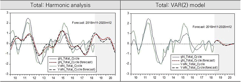
In our analysis, if we use the parameters estimated in the harmonic analysis, we could forecast long-term common cycles embedded in the time series of gN and VolN after 11.2018. And then, if we use the parameters estimated in the VAR model, we could also forecast long-term movements of cyclical components in the time series of gN and VolN after 11.2018.
If we compare the forecasted values generated by using harmonic analysis and VAR model, we could get more reasonable projection about the environment of future housing market.
In the aspect of long-term common cycles in gN and VolN in whole country, we could confirm that the movement of trading volume slightly precedes that of housing price change rates. The long-term common cycles in both gN and VolN had upward movement from trough to peak during 2018. But, the movement direction is forecasted to be changed from peak to trough after 2019 to the end of 2020. The forecast values from VAR(2) model also show downward direction after 2019.
What to think about when interpreting the cycle analysis results of this study is the point that the housing price has long term upward trend.8) Therefore, it should be interpreted that lowering after the cycle reaches its peak does not mean a recession in the housing market or a decline in housing prices, but at this point, housing prices still rise but the speed of increase decreases relatively. Conversely, it can be interpreted that when the cycle reaches its trough and then switches to the peak direction, the volume of transactions increases, followed by a relatively faster speed of increase in housing prices.

Considering these point, combining the forecast results of harmonic analysis and VAR(2) model, the housing market is expected to face a slow speed of increase in housing sales prices for the time being after 2019. But after the end of 2020, housing price is expected to be switched to a relatively rapid increase again.
In the aspect of long-term common cycles in gN and VolN in SMetro, we could also confirm that the movement of trading volume slightly precedes that of housing price change rates. The long-term common cycles in both gN and VolN had upward movement from trough to peak during 2018. But, the movement direction is forecasted to be changed from peak to trough after 2019 to the end of 2020. The results in SMetro are similar to those in whole country. The forecast values from VAR(4) model also show downward direction after 2019 and the speed of downward in Smetro is faster than that in whole country.
Combining the forecast results of harmonic analysis and VAR(4) model, it is expected that the housing market in the metropolitan area will face a slow speed of increase in housing price for the time being after 2019. But after the end of 2020, housing price is expected to be switched to a relatively rapid increase again.

In the aspect of long-term common cycles in gN and VolN in 5Cities, we could also confirm that the movement of trading volume slightly precedes that of housing price change rates. The long-term common cycles in both gN and VolN had upward movement from trough to peak during 2017 to 2019. But, the movement direction is forecasted to be changed from peak to trough after the middle of 2019 to the end of 2020. The forecast values from VAR(3) model also show downward diretion after the middle of 2019 but the magnitude of downward is expected not so significant because the recent amplitude of the cycles was relatively small in 5Cities.
Combining the forecasted results of harmonic analysis and VAR(3) model, it is expected that the housing market in the 5 big cities will face a slow speed of increase in housing price for the time being after 2019. But after the end of 2020, housing price is expected to be switched to a relatively rapid increase again. The results in 5 big cities also are similar to those in whole country.


In the aspect of long-term common cycles in gN and VolN in NMetro, we could confirm that the two variables move similarly but could not say that the movement of trading volume precedes that of housing price change rates. The long-term common cycles in both gN and VolN had upward trends after 2018. But, the movement direction is forecasted to be changed from peak to trough after the middle of 2020. The forecasted values from VAR(3) model also show downward direction after the middle of 2019 but the magnitude of upward or downward is expected not so significant because the recent amplitude of the cycles was relatively small in NMetro area.
Combining the forecast results of harmonic analysis and VAR(3) model, it is expected that the movement of housing prices in another housing market slightly precedes that in NMetro housing market. This result implies that regional housing markets can be devided into several submarkets.
Ⅳ. Conclusion
We can say that the movements of housing prices and trading volume have long-term cycles. So, we can presume that there would be a close relationship between cyclic components embedded in these two variables. But, until now, it is difficult to find studies which analyzed cyclical characteristics and the relationship in the aspect of common cycles embedded in these two variables. In this analysis, unlike the previous studies conducted to confirm the correlation and lead-lag relationship between housing prices and trading volume using the methodologies in time domain analysis, we tried to interpret from different points of view through analyzing cyclical characteristics embedded in these two variables by using spectral analysis in frequency domain. When we forecast cycles in housing prices and trading volume, for the purpose of comparison, we added the results of VAR(p) model analysis in time domain in addition to the results of the spectral analysis in frequency domain. After identifying common cycles embedded in these two variables, we could confirm a close relationship in the aspect of common cycles. And then, we could confirm the current position of two variables in the aspect of long-term cycles and could forecast future direction of the cycles.
In our analysis, we could confirm that the movement of trading volume slightly precedes that of housing price change rates. The long- term common cycles in both time series had upward movement from trough to peak during 2018. But, the movement direction is forecasted to be changed from peak to trough after 2019 to the end of 2020. Considering the point that the housing price has long term upward trend, it should be interpreted that lowering after the cycle reaches its peak does not mean a recession in the housing market or a decline in housing prices, but at this point, housing prices still rise but the speed of increase decreases relatively. And when the cycle reaches its trough and then switches to the peak direction, we can say that the volume of transactions increases, followed by a relatively faster speed of increase in housing prices. So, the results of our analysis show that housing market was expected to face a slow speed of increase in housing prices while decrease in trading volume for the time being after 2019. But after the end of 2020, both trading volume and housing price were expected to be switched to a relatively rapid increase again.
Meanwhile, in our analysis, we used the data from 2007.01-2018.10 and showed the forecast result after 11.2018. So, by passage of time, it is necessary to conduct the analysis periodically with updated data. Plus, it is also necessary to conduct spectral analysis to confirm the relationship among housing price, trading volume, and other variables such as interest rate at the same time. Ultimately, as we can see from the results of this analysis, we could improve the rationality about the forecasting results of future cycles by confirming the results from time domain and frequency domain analysis concurrently.


